Tempo Change JND Experiment

This webpage describes an experiment to determine the minimum uniform acceleration or ritard which is perceivable over a fixed number of beats. The minimum just noticeable differences (JNDs) in tempo can then be used to model the perception of tempo changes in actual performances.

JNDs can be measured using a two-interval forced-choice test. A person chooses whether a stimulus is one of two types. If the listener can distinguish very well between the categories, the responses for the identification of the stimulus will be 100% correct. If the person cannot distinguish between the two categories of stimuli, the identification rate will be at 50% (provided that the stimuli are presented using a uniform random selection process such as flipping a coin).

The JND is usually defined as the point at which a person can generate a 75% accurate rate for the stimuli. If someone can correctly identify the two categories 3 out of 4 times, then they are just barely able to accurately distinguish between the two groups, and it is unlikely that they are guessing the correct answers purely by chance.

In this experiment, the JND values for tempo changes are measured. The two stimuli are a constantly increasing tempo, and a constantly decreasing tempo. And this experiment measures how small these contrasting tempo changes can be distinguished from each other given a certain number of beats over which the tempo change occurs. It is expected that given fewer numbers of clicks in the soundfile, the tempo change must be greater than for larger numbers of clicks in order for a tempo change to be perceived.

Experimental setup

The test material consists of a sound file which contains a certain number of clicks. Each click consists of one millisecond of white noise (44 samples at 44100 Hz sampling rate). Each click is not identical but rather independent portions of white noise. This causes slight loudness and pitch variations between clicks. Each trial sound was generated with a unique random noise content, which were not repeated in subsequent sound files.

Listeners are asked to identify whether the soundfile contains clicks which are speeding up in tempo, or slowing down in tempo. The change in tempo is controlled by a constant multiplicative factor. For example, if that factor were 0.01 (1%), and the duration between the first two clicks were 1000 milliseconds, then the next click will occur after 1010 milliseconds if the tempo is slowing down, or it will occur after 990 milliseconds if the tempo is speeding up.

For the current experiment, a fixed starting tempo of 1000 milliseconds (a tempo of 60 beats per minute) was used for all sound tests.

The conditions for acquiring the data for the experiment are:

The listener usually listened to a randomly selected tempo change at a known fixed magnitude for 40 consecutive trials.
The listener wrote down whether the tempo was perceived as speeding up or slowing down.
The correct answer was then revealed to the listener. This allowed the listener to learn the correct answer as the tests progressed and can be seen somewhat in the results.
The soundfile was played only once and the listener then gave an answer. This was to prevent cheating by listening to the larger tempo change from the end of the sound back to the beginning of the sound, which is larger than the individual beat tempo changes as the sound sample progresses. However, sometimes a second hearing was allowed for the 3-click trials, since there is no advantage for this case.

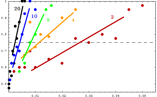
Results

Shown below is a plot of the accuracy for distinguishing between an acceleration or ritard of equivalent magnitude. Identification accuracy for 5 lengths of clicks were done: 3, 4, 5, 10 and 20 clicks. The vertical axis displays the fraction of correct answers, and the horizontal axis plots the fractional change between beats (either slower or faster).

The straight lines on the plot are interpretive (drawn by hand to fit a line through the points around the 75% accuracy rate), and they measure the approximate average crossing points for reading the JND values from the plot:

clicks:	3	4	5	10	20
JND:	0.0265	0.0115	0.0082	0.0040	0.0024
faster end delta:	-26.5	-34.4	-48.9	-142.7	-404.9
slower end delta:	26.5	34.6	49.5	145.3	416.0
faster end tempo:	63.3	62.1	62.0	62.2	62.8
slower end tempo:	56.9	57.0	58.0	57.9	57.3

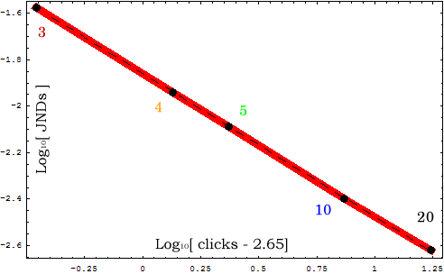
The faster end delta is the difference in milliseconds between time of the last beat if the tempo of the first beat is held constant and the actual last time for the given acceleration. The slower end delta is the same thing for a slowing tempo.

The faster end tempo is the tempo marking in beats per minute of the last beat in the click sequence, and the slower end tempo is the same for ritards.

What the above table means, is that if you increase the tempo by 3% each beat, a person (at least the one who took the test) can perceive the acceleration in tempo. If the tempo is changed by 1% for each beat, then a tempo will not be perceptible until at least 5 beats (including the ones used to define the starting tempo).

The most effective method to identify tempo changes particular for a small number of beats, seemed to be to subdivide the beat into 4 (or 2) subdivisions either mentally or physically (tapping) and then analyzing whether the soundfile speed up or slowed down compared to those subdivisions. In many tests a tempo acceleration felt sligtly stronger than an equivalent magnitude ritard.

If you take the log of both the JND values, and the number of clicks (with an offset of -2.65), the values fall very well into a straight line. Don't know why the offset of -2.65, but would expect an offset of either -1 (for example 3 clicks equals 2 tempo regions), or -2 (for example 3 clicks equals one defining tempo region, and one tempo change region). The -0.6 offset could just be due to noise, or some other smaller perceptual or memory effect.

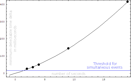
Basically, the slope of the above plot (-0.62) allows a prediction of the tempo JND for other lengths of clicks (accurate at least within the range between 3 and 20 clicks). If you increase the number of clicks by 10 times, you will decrease the tempo JND factor by 4 times.

Also, the above plot indicates that tempo perception occurs in a log space just like pitch and loudness. Tempo perception most likely occurs cognatively since it involves memory and prediction in some way, while pitch and loudness JNDs are more related to the properties of the measuring device (the ear) rather than to higher brain functions.

Here is another plot which shows the minimum time delta due to tempo changes as a function of time in seconds for the duration of the duration of the clicks. The data points fit well onto a parabolic curve. The blue line shows the minimum time difference at which the order of two events can be detected (so it is not really possible to have any meaningful data points below this line).

If trials (for larger numbers of clicks) start generating points below this curve, then that would be a good case that absolute tempo perception is kicking in. Here is a table of the predicted slower delta times in milliseconds for various click lengths at the predicted JND points in the above plot:

clicks	end offset
3	23.2
4	36.9
5	51.8
6	67.8
7	85.1
8	103.5
9	123.1
10	143.8
11	165.8
12	188.9
13	213.2
14	238.7
15	265.3

clicks	end offset
16	293.2
17	322.2
18	352.4
19	383.7
20	416.3
25	596.6
30	806.4
35	1045.6
40	1314.3
45	1612.3
50	1939.9
55	2296.9
60	2683.3

clicks	end offset
65	3099.1
70	3544.4
75	4019.1
80	4523.2
85	5056.8
90	5619.8
95	6212.3
100	6834.1
150	14671.8
200	25452.9
250	39177.5
300	55845.6
350	75457.1

clicks	end offset
400	98012.1
450	123510.5
500	151952.4
550	183337.7
600	217666.6
650	254938.8
700	295154.6
750	338313.8
800	384416.4
850	433462.5
900	485452.1
950	540385.1
1000	598261.6

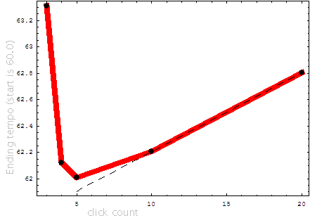
The next plot compares the final tempo (for acceleration JNDs) between the last two clicks in a sequence and the length of the sequence. It looks like the plot shows the effects of short-term memory. For short sequences, the plot increases in sensitivity to the tempo change, reaching maximum sensitivity around 6 clicks (5 tempo intervals). For longer click counts, the tempo sensitivity decreases due to a more gradual shift to the final JND tempo. It is expected that this curve will flatten out for larger click counts. For example, if there were a test with 1000 clicks, the current plot would predict a final tempo of 120 beats per minute. However, using an absolute sense of tempo, you should be able to distinguish between 60 and 120 beats per minute. Therefore memory will not be the most important factor for very long click counts.

Raw Data

Here are the set of files used to create the first figure. Each click count set is in a separate file:

The data forms six columns:

**beats -- the number of clicks present in the test soundfile.
**tempo -- the starting tempo between the first two clicks.
**gain -- the fractional increase or decrease in the duration between each click.
**ans -- the human-provided answer.
**type -- the actual type of tempo change present in the test soundfile.
**corr -- Y if the answer was correct, N if the answer was incorrect.

These raw data files were then processed with a PERL program to calculate the error rates for each click count and gain type. The resulting error rates for each click count/gain were then analyzed in a Mathematica notebook:

Further Work

Since performers cannot play with a time accuracy as good as a computer, there will be random offsets in the tempo when the performer is (1) trying to keep the tempo constant, (2) trying to accelerate, and (3) trying to ritard. Another experiment will be done to measure the perception of tempo changes when the click timings are displaced from their exact positions by Gaussian noise. It also might be interesting to measure the resolution of "absolute tempo".

Further Reading

Looking at perception of continuous tempo drift: A new method for estimating internal drift and just noticeable difference by Sofia Dahl and Svante Granqvist in the Proceedings of the Stockholm Music Acoustics Conference, August 6-9, 2003, Stockholm, Sweden.
Human Preferences for Tempo Smoothness by Emilios Cambouropoulos, Simon Dixon, Werner Goebl and Gerhard Widmer. 7th International Symposium on Systematic and Comparative Musicology, 16-19 August 2001, Jyvaskyla, Finland. pp. 18-26.